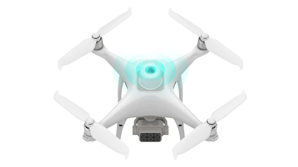
Let’s look at some imagery collected from DJI’s P4M setup released last year. It’s being sold as a full agricultural solution. The Phantom 4 Multispectral (P4M) is shipping with one RGB camera and five narrow band sensors, including red edge and near infrared.
That’s quite the sensor array. Sensors are coming down in price, a lot with the push towards self driving vehicles I’d expect this trend to continue. Meaning this model ships for $6,499 USD.
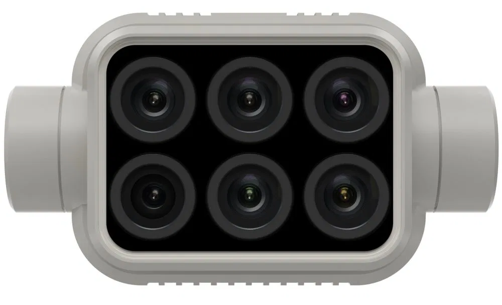
Sensor Basics
To give some reality to this think about the sensor above, each is capturing a different snapshot of the environment. Only one of the 6 sensors is capturing the world as we would recognise it, in a Red, Green and Blue composite.
The RGB sensor tangent
In order to capture the world in RGB we use filters over the array arranged into a pattern arranged to mimic the way the human eye captures information. (Thank you Wikipedia). This particular arrangement was invented by Bruce Bayers in the 1970’s. It filters for twice as many green filters to red or blue to mimic the human eye.

While there is no real need to understand physics it is interesting to understand a little about how sensors work to collect data.

Practical Application
This means that when we collect imagery using P4M you are going to capture a lot of data. Each snapshot of the environment is actually 6 images.
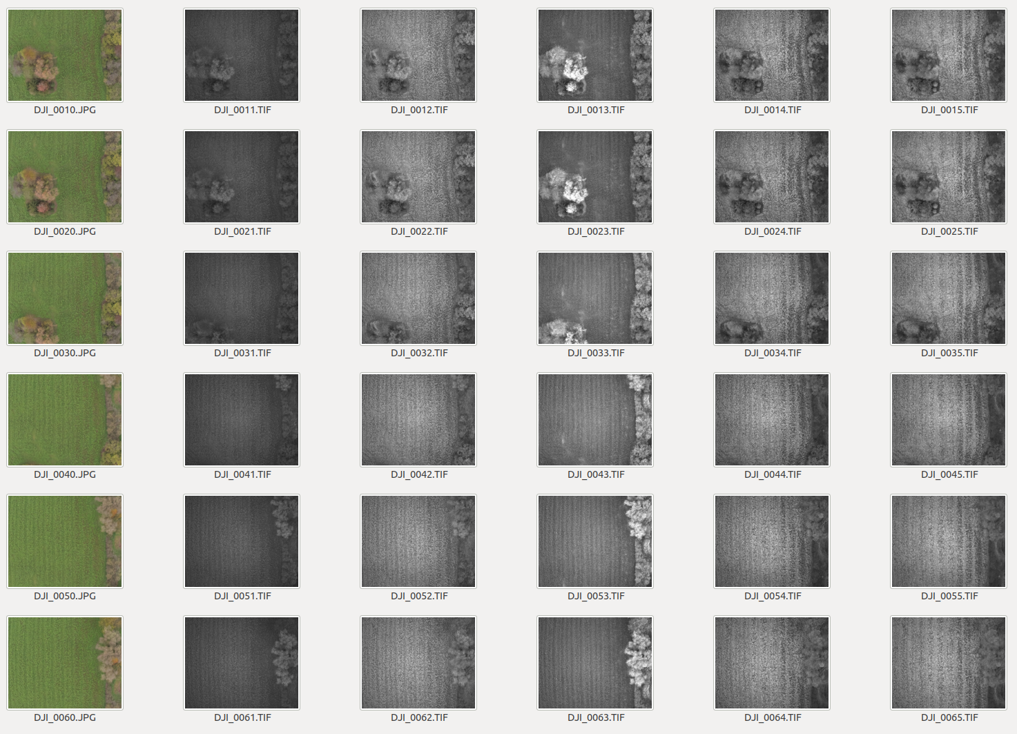
The Rigg
We refer to this setup, multiple image captures per snapshot, as the Rigg. In theory all 6 images should be taken at the same time. Errors happen and sometimes it seems that one of the sensors captures data a little later than the rest.
But the other possibility is that one of the 6 sensors fails to capture while the other five succeed.
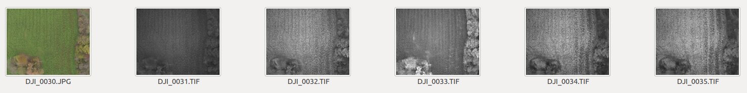
Reading the Data
If the Rigg fails to capture the exact number of expected images my processing of these images into a Geospatial Product is going to fail. This is hard. You cannot just rely on GDAL or Rasterio to do the work for you I’m afraid. Multispectral cameras that I’m familiar with don’t tend to write carefully like satellite imagery because they don’t have respective tiff tags or even are just writing .jps, which have no alternative to tiff tags.
Reading XMP metadata
Alas you need to read the XMP metadata, which means you need access to some C++ libraries which are specifically able to access this data. Fortunately there is a python module that has bindings to exiv2, the C++ library for manipulation of EXIF, IPTC and XMP image metadata.
from pyexiv2 import Image
img = Image(path)
data = img.read_exif()
print(data)
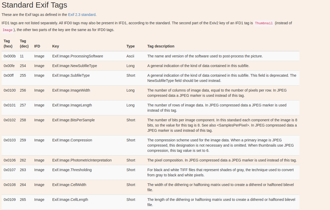
img.close()As a subject this one is quite new to me. There are many useful posts on the subject. Here’s one who uses the Python Image Library, but alas I could not get what I wanted from it. Nevertheless, it is a well written blog, here is the link incase you find it useful, and critically it also contains a link to the exif documentation which was very helpful for me to understand what I’m actually trying to access. While learning about how images are encoded a whole new world of detail opened up to me reading through this specification table.
Reading XMP Camera Bandname
After learning more about how XMP data is encoded in C++ I found myself reading through the available metadata of the Camera setup.
Xmp.Camera.RigName
Xmp.Camera.BandName
Xmp.Camera.CentralWavelength
Xmp.Camera.WavelengthFWHM
Xmp.Camera.ModelType
Xmp.Camera.PrincipalPoint
Xmp.Camera.PerspectiveFocalLength
Xmp.Camera.PerspectiveFocalLengthUnits
Xmp.Camera.PerspectiveDistortion
Xmp.Camera.VignettingCenter
Xmp.Camera.VignettingPolynomial
Xmp.Camera.BandSensitivity
Xmp.Camera.RigRelatives
Xmp.Camera.RigCameraIndex
Xmp.Camera.RigRelativesReferenceRigCameraIndex
Xmp.Camera.GPSXYAccuracy
Xmp.Camera.GPSZAccuracy
Xmp.Camera.Irradiance
Xmp.Camera.IrradianceYaw
Xmp.Camera.IrradiancePitch
Xmp.Camera.IrradianceRoll
Xmp.MicaSense.BootTimestamp
Xmp.MicaSense.RadiometricCalibration
Xmp.MicaSense.ImagerTemperatureC
Xmp.MicaSense.FlightId
Xmp.MicaSense.CaptureId
Xmp.MicaSense.TriggerMethod
Xmp.MicaSense.PressureAlt
Xmp.MicaSense.DarkRowValue
Xmp.DLS.Serial
Xmp.DLS.SwVersion
Xmp.DLS.CenterWavelength
Xmp.DLS.Bandwidth
Xmp.DLS.TimeStamp
Xmp.DLS.SpectralIrradiance
Xmp.DLS.HorizontalIrradiance
Xmp.DLS.DirectIrradiance
Xmp.DLS.ScatteredIrradiance
Xmp.DLS.SolarElevation
Xmp.DLS.SolarAzimuth
Xmp.DLS.EstimatedDirectLightVector
Xmp.DLS.Yaw
Xmp.DLS.Pitch
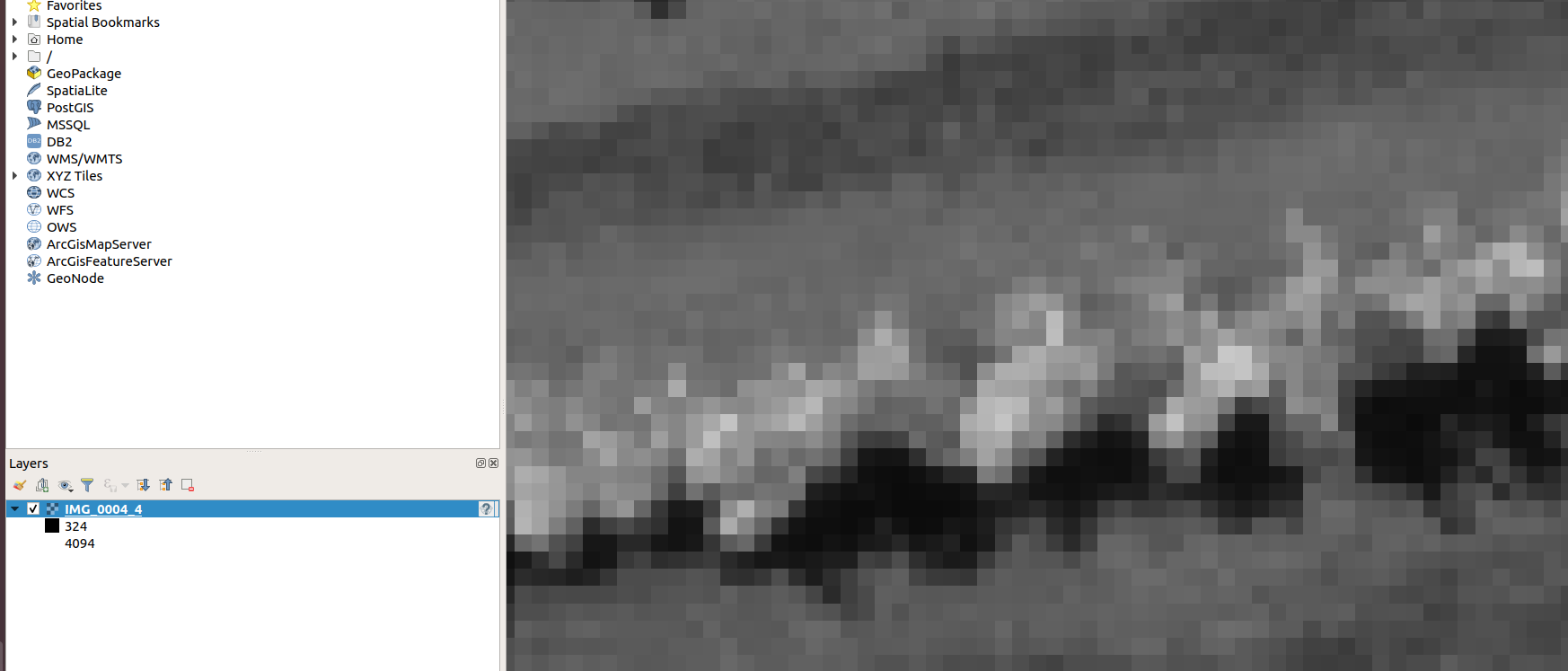
Xmp.DLS.RollUltimately this lead me to the answer to my question, the name of the image band I’ve been looking at in a grayscale image is “NIR”
Here’s the code snippet, but do keep in mind that the version of pyexiv2 is very important and be prepared to debug this one yourself, it took me a while to get the correct methods.
from pyexiv2 import Image
img = Image(path)
data = img.read_exif()
data = (img.read_xmp())

# This will list all the available data
data = dir(img)
for i in data:
   print((i))

# This will tell you the band name of the image
print(data["Xmp.Camera.BandName"])
img.close()
Thanks for reading.

Leave a comment